2.7 Linear system representation

Linear systems are treated as specific typed lists tlist. The basic function which is used for defining linear systems is syslin. This function receives as parameters the constant matrices which define a linear system in state-space form or, in the case of system in transfer form, its input must be a rational matrix. To be more specific, the calling sequence of syslin is either Sl=syslin('dom',A,B,C,D,x0) or Sl=syslin('dom',trmat). dom is one of the character strings 'c' or 'd' for continuous time or discrete time systems respectively. It is useful to note that D can be a polynomial matrix (improper systems); D and x0 are optional arguments. trmat is a rational matrix i.e. it is defined as a matrix of rationals (ratios of polynomials). syslin just converts its arguments (e.g. the four matrices A,B,C,D) into a typed list Sl. For state space representation Sl is the tlist(['lss','A','B','C','D'],A,B,C,D,'dom'). This tlist representation allows to access the A-matrix i.e. the second entry of Sl by the syntax Sl('A') (equivalent to Sl(2)). Conversion from a representation to another is done by ss2tf or tf2ss. Improper systems are also treated. syslin defines linear systems as specific tlist. (help syslin).

 
-->//list defining a linear system
 
-->A=[0 -1;1 -3];B=[0;1];C=[-1 0];
 
-->Sys=syslin('c',A,B,C)
 Sys  =
 
 
       Sys(1)   (state-space system:)
 
!lss  A  B  C  D  X0  dt  !
 
       Sys(2) = A matrix = 
 
!   0.  - 1. !
!   1.  - 3. !
 
       Sys(3) = B matrix = 
 
!   0. !
!   1. !
 
       Sys(4) = C matrix = 
 
! - 1.    0. !
 
       Sys(5) = D matrix = 
 
    0.  
 
       Sys(6) = X0 (initial state) = 
 
!   0. !
!   0. !
 
       Sys(7) = Time domain = 
 
 c   
 
-->//conversion from state-space form to transfer form
 
-->Sys('A')  //The A-matrix
 ans  =
 
!   0.  - 1. !
!   1.  - 3. !
 
-->Sys('B')
 ans  =
 
!   0. !
!   1. !
 
-->hs=ss2tf(Sys)
 hs  =
 
        1        
    ---------    
              2  
    1 + 3s + s   
 
-->size(hs)
 ans  =
 
!   1.    1. !
 
-->hs('num')
 ans  =
 
    1   
 
-->hs('den')
 ans  =
 
              2  
    1 + 3s + s   
 
-->typeof(hs)
 ans  =
 
 rational   
 
-->//inversion of transfer matrix
 
-->inv(hs)
 ans  =
 
              2  
    1 + 3s + s   
    ----------   
        1        
 
-->//inversion of state-space form
 
-->inv(Sys)
 ans  =
 
 
       ans(1)   (state-space system:)
 
!lss  A  B  C  D  X0  dt  !
 
       ans(2) = A matrix = 
 
     []
 
       ans(3) = B matrix = 
 
     []
 
       ans(4) = C matrix = 
 
     []
 
       ans(5) = D matrix = 
 
              2  
    1 + 3s + s   
 
       ans(6) = X0 (initial state) = 
 
     []
 
       ans(7) = Time domain = 
 
 c   
 
-->//converting this inverse to transfer representation
 
-->ss2tf(ans)
 ans  =
 
              2  
    1 + 3s + s

The list representation allows manipulating linear systems as abstract data objects. For example, the linear system can be combined with other linear systems or the transfer function representation of the linear system can be obtained as was done above using ss2tf. Note that the transfer function representation of the linear system is itself a tlist. A very useful aspect of the manipulation of systems is that a system can be handled as a data object. Linear systems can be inter-connected , their representation can easily be changed from state-space to transfer function and vice versa.

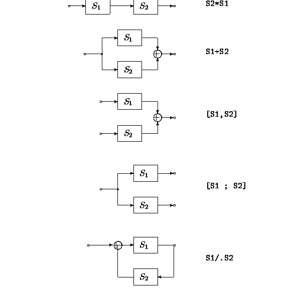
The inter-connection of linear systems can be made as illustrated in Figure 2.1.

  

Figure 2.1: Inter-Connection of Linear Systems

For each of the possible inter-connections of two systems S1 and S2 the command which makes the inter-connection is shown on the right side of the corresponding block diagram in Figure 2.1. Note that feedback interconnection is performed by S1/.S2.

The representation of linear systems can be in state-space form or in transfer function form. These two representations can be interchanged by using the functions tf2ss   and ss2tf   which change the representations of systems from transfer function to state-space and from state-space to transfer function, respectively. An example of the creation, the change in representation, and the inter-connection of linear systems is demonstrated in the following Scilab session.

 
-->//system connecting
 
-->s=poly(0,'s');
 
-->S1=1/(s-1)
 S1  =
 
      1     
    -----   
  - 1 + s   
 
-->S2=1/(s-2)
 S2  =
 
      1     
    -----   
  - 2 + s   
 
-->S1=syslin('c',S1);
 
-->S2=syslin('c',S2);
 
-->Gls=tf2ss(S2);
 
-->ssprint(Gls)
 
.           
x = | 2 |x + | 1 |u   
 
y = | 1 |x   
 
-->hls=Gls*S1;
 
-->ssprint(hls)
 
.   | 2  1 |    | 0 |
x = | 0  1 |x + | 1 |u   
 
y = | 1  0 |x   
 
-->ht=ss2tf(hls)
 ht  =
 
        1        
    ---------    
              2  
    2 - 3s + s   
 
-->S2*S1
 ans  =
 
        1        
    ---------    
              2  
    2 - 3s + s   
 
-->S1+S2
 ans  =
 
    - 3 + 2s     
    ----------   
              2  
    2 - 3s + s   
 
-->[S1,S2]
 ans  =
 
!     1         1    !
!   -----     -----  !
! - 1 + s   - 2 + s  !
 
-->[S1;S2]
 ans  =
 
!     1    !
!   -----  !
! - 1 + s  !
!          !
!     1    !
!   -----  !
! - 2 + s  !
 
-->S1/.S2
 ans  =
 
    - 2 + s      
    ---------    
              2  
    3 - 3s + s   
 
-->S1./(2*S2)
 ans  =
 
  - 2 + s    
    -----    
  - 2 + 2s

The above session is a bit long but illustrates some very important aspects of the handling of linear systems. First, two linear systems are created in transfer function form using the function called syslin  . This function was used to label the systems in this example as being continuous (as opposed to discrete). The primitive tf2ss is used to convert one of the two transfer functions to its equivalent state-space representation which is in list form (note that the function ssprint creates a more readable format for the state-space linear system). The following multiplication of the two systems yields their series inter-connection. Notice that the inter-connection of the two systems is effected even though one of the systems is in state-space form and the other is in transfer function form. The resulting inter-connection is given in state-space form. Finally, the function ss2tf is used to convert the resulting inter-connected systems to the equivalent transfer function representation.