 |
xstring : draws a string or a matrix of strings
xstringl : computes a rectangle which surrounds
a string
xstringb : draws a string in a specified box
xnumb : draws a set of numbers
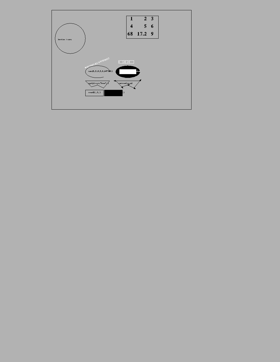
We give now the sequence of the commands for obtaining the figure 5.8.
//	initialize default environment variables
xset('default');
xset("use color",0);
plot([1:10]);
xbasc()
xrect(0,1,3,1)
xfrect(3.1,1,3,1)
xstring(0.5,0.5,"xrect(0,1,3,1)")
xstring(4.,0.5,"xfrect(3.1,1,3,1)")
xset("alufunction",6)
xstring(4.,0.5,"xfrect(3.1,1,3,1)")
xset("alufunction",3)
xv=[0 1 2 3 4]
yv=[2.5 1.5 1.8 1.3 2.5]
xpoly(xv,yv,"lines",1)
xstring(0.5,2.,"xpoly(xv,yv,""lines"",1)")
xa=[5 6 6 7 7 8 8 9 9 5]
ya=[2.5 1.5 1.5 1.8 1.8 1.3 1.3 2.5 2.5 2.5]
xarrows(xa,ya)
xstring(5.5,2.,"xarrows(xa,ya)")
xarc(0.,5.,4.,2.,0.,64*300.)
xstring(0.5,4,"xarc(0.,5.,4.,2.,0.,64*300.)")
xfarc(5.,5.,4.,2.,0.,64*360.)
//xset("alufunction",6)
xclea(5.6,4.4,2.8,0.8);
xstring(5.8,4.,"xfarc  and then  xclea")
//xset("alufunction",3)
xstring(0.,4.5,"WRITING-BY-XSTRING()",-22.5)
xnumb([5.5 6.2 6.9],[5.5 5.5 5.5],[3 14 15],1)
isoview(0,12,0,12)
xarc(-5.,12.,5.,5.,0.,64*360.)
xstring(-4.5,9.25,"isoview + xarc",0.)
xset("font",4,5)
A=["  1" "       2" "  3";"  4" "       5" "  6";"68" "  17.2" "  9"];
xstring(7.,10.,A);
rect=xstringl(7,10,A);
xrect(rect(1),rect(2),rect(3),rect(4));
Figdirfigures/
e have seen that some parameters of the graphics are controlled by a graphic context ( for example the line thickness) and others are controlled through graphics arguments .
(i)-xset("use color",flag) changes to color or gray plot according to the values (1 or 0) of flag.
(ii)-xset("window",window-number) sets the current window to the window window-number and creates the window if it doesn't exist.
(iii)-xset("wpos",x,y) fixes the position of the upper left point of the graphic window.
The choice of the font, the width and height of the window, the driver... can be done by xset.