Bergische Universität Wuppertal
Fachbereich Mathematik und Naturwissenschaften
Angewandte Mathematik - Numerische Analysis (AMNA)

People
Research
Publications
Teaching


Anton Arnold , Matthias Ehrhardt , Ivan Sofronov
Discrete transparent boundary conditions for the 1D Schrödinger equation

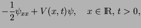
  • scaled Schrödinger equation:
    $\displaystyle i\psi_t \!\!$ $\displaystyle =$ $\displaystyle -\frac{1}{2}\psi_{xx}+V(x,t)\psi,
\quad x\in{\ensuremath{\mathrm{I}\!\mathrm{R}}},\,t>0,$  
    $\displaystyle \psi(x,0) \!\!$ $\displaystyle =$ $\displaystyle \psi^I(x),$   supp $\displaystyle \psi^I\subset[0,X]$  

with

$\displaystyle V(x,t)=V_-\equiv \co$   for $\displaystyle x\le0,\,t\ge0,
$
$\displaystyle V(x,t)=V_+ \equiv \co$   for $\displaystyle x\ge X,\,t\ge0
$
  • goal: Solve the whole space problem (almost) exactly on the computational interval $ [0,X]$ by introducing transparent boundary conditions at $ x=0,\,x=X$.

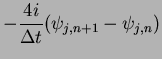
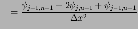
  • Crank-Nicolson finite difference scheme:
    grid points: $ x_j=j\Delta x$ (with $ J\Delta x=X$), $ t_n=n\Delta t$
    approximation: $ \psi_{j,n}\sim\psi(x_j,t_n), \,j\in{\ensuremath{\mathrm{Z}\!\!\mathrm{Z}}},\,n\in\ensuremath{\mathrm{I}\!\mathrm{N}}_0$$ V_{j,n+\frac{1}{2}}=V(x_j,t_{n+\frac{1}{2}})$
    numerical scheme for whole space problem:
        $\displaystyle -\frac{4i}{\Delta t}(\psi_{j,n+1}-\psi_{j,n})$  
        $\displaystyle \quad=\frac{\psi_{j+1,n+1}-2\psi_{j,n+1}+\psi_{j-1,n+1}}{\Delta x^2}$$\displaystyle \quad+\,\frac{\psi_{j+1,n}-2\psi_{j,n}+\psi_{j-1,n}}{\Delta x^2}$          (1)
        $\displaystyle \quad- 2V_{j,n+\frac{1}{2}}\left(\psi_{j,n+1}+\psi_{j,n}\right),
\qquad j\in{\ensuremath{\mathrm{Z}\!\!\mathrm{Z}}},\,n\ge0,$  
     

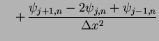
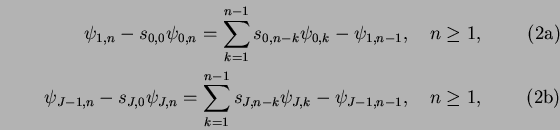
  • discrete transparent boundary conditions:  
    (to be used with scheme (1) on $ 1\le j\le J-1$)
    \begin{subequations}\begin{align}
 \psi_{1,n}-s_{0,0}\psi_{0,n}=\sum_{k=1}^{n-1}...
..._{J,n-k}\psi_{J,k}-\psi_{J-1,n-1},
 \quad n\ge 1,
 \end{align}\end{subequations}

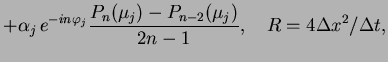
    with convolution kernels $ \{s_{0,n}\},\,\{s_{J,n}\}$:
    $\displaystyle s_{j,n}=\!\!\!\!\!\!\!\!$   $\displaystyle \Bigl[1-i\frac{R}{2}+\frac{\sigma_j}{2}\Bigr]\delta_{n,0}
+\Bigl[1+i\frac{R}{2}+\frac{\sigma_j}{2}\Bigr]\delta_{n,1}$  
        $\displaystyle +\alpha_j\,e^{-in\varphi_j}\frac{P_n(\mu_j)-P_{n-2}(\mu_j)}{2n-1}, \quad
R=4\Delta x^2/\Delta t,$  
$\displaystyle \varphi_j=\arctan\frac{2R(\sigma_j+2)}{R^2-4\sigma_j-\sigma_j^2},...
...2+4\sigma_j+\sigma_j^2}{\sqrt{(R^2+\sigma_j^2)\bigl[R^2+(\sigma_j+4)^2\bigr]}},$    
$\displaystyle \sigma_j=2\Delta x^2 V_j,
 \quad\alpha_j=\frac{i}{2}\sqrt[4]{(R^2+\sigma_j^2)\bigl[R^2+(\sigma_j+4)^2\bigr]}\,e^{i\varphi_j/2},
 \quad j=0,J.$    
$ P_n$ ... Legendre polynomials ( $ P_{-1}\equiv P_{-2}\equiv0$)

initial condition must satisfy: $ \psi_{0,0}=\psi_{1,0}=\psi_{J-1,0}=\psi_{J,0}=0$


REMARK:
The evaluation of the convolutions (2) is very expensive for large-time calculations $ \Rightarrow$ 
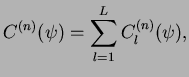
approximative "sum-of-exponential'' convolution coefficients strongly reduce the numerical effort.


  • approximative transparent boundary conditions:
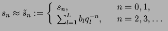
    $\displaystyle s_n \approx \tilde{s}_n:=\left\{
 \begin{array}{lcl}
 s_n, &&n=0,1,\\
 \sum_{l=1}^L b_l q_l^{-n},&&n=2,3,\dots
 \end{array}
 \right.$                                       (3)

    $ L\in\ensuremath{\mathrm{I}\!\mathrm{N}}$ ... parameter to choose
    Java-applet for calculation of $ s_0,\,s_1$, $ \{b_l,\, q_l\}$ for given $ \Delta x,\,\Delta t, \,V,\,L$ 
    download Maple-code for calculation of$ \{s_n\},\, \{\tilde{s}_n\}$


  • fast evaluation of discrete convolutions: For the "sum-of-exponential'' convolution coefficients (3) the resulting convolution in (2):

    $\displaystyle C^{(n)}(\psi):=\sum_{k=1}^{n-2}\tilde{s}_{n-k}\psi_{k},\quad n\ge 3
$

    can be computed very efficiently by the algorithm:

    $\displaystyle C^{(n)}(\psi)=\sum_{l=1}^{L} C_l^{(n)}(\psi),$    
    where
        $\displaystyle C_l^{(2)}(\psi) \equiv 0,$  
        $\displaystyle C_l^{(n)}(\psi)=q_l^{-1} C_l^{(n-1)}(\psi)+b_lq_l^{-2}\psi_{n-2},
\quad\quad n=3,4,\dots$  

  • example - free Schrödinger equation:  
    Gaussian beam, travelling right


Solution with L=10:


Solution with L=20:

[Preprint: Arnold - Ehrhardt - Sofronov '02]


University of Wuppertal
Faculty of Mathematics and Natural Sciences
Department of Mathematics
Applied Mathematics & Numerical Analysis Group

Last modified:   Disclaimer   ehrhardt@math.uni-wuppertal.de